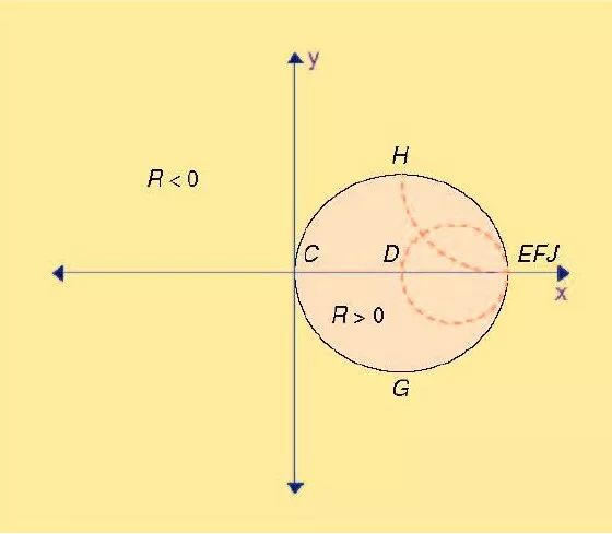
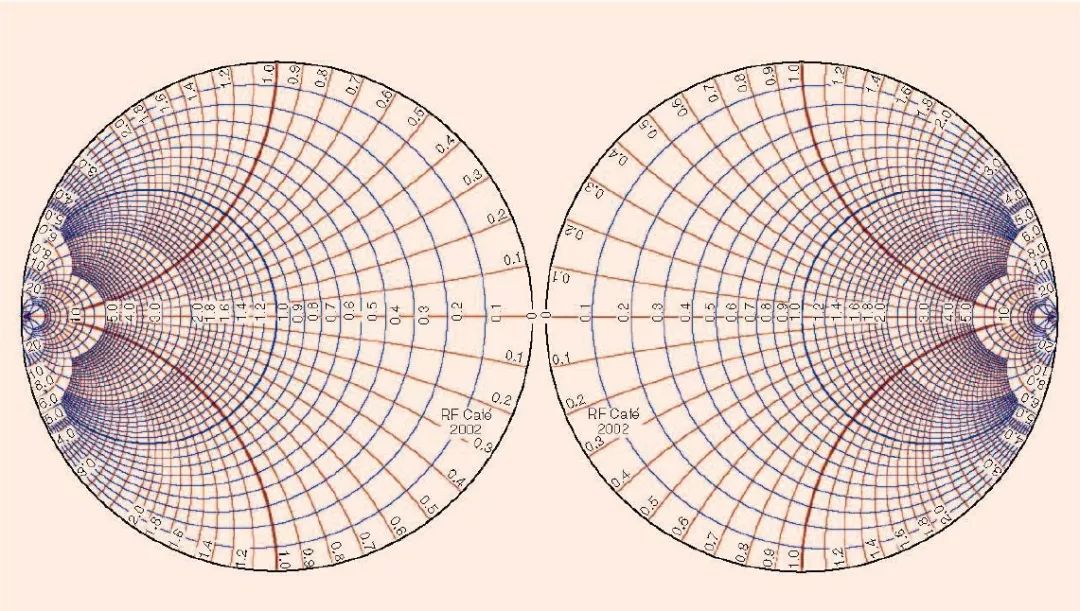
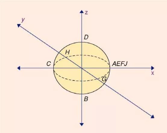
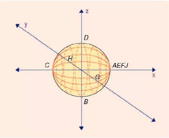
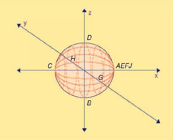
Before Christopher Columbus sailed, everyone thought the earth was flat... Over the past many years, I have extended the traditional Smith chart to help me understand the issues related to negative impedance devices such as oscillator design and amplifier stability in the RF field. Its concept makes me have a deeper understanding of the nature of the problems related to impedance, and also proves that this is a very useful additional design aid. Recently, when I discussed with other engineers at the dinner table, I mentioned some of my own ideas. These ideas have been recognized by everyone. Since then, they have repeatedly persuaded me to publish my own extension of the Smith Chart. For this reason, in this article, I tried to explain the idea behind the conceptual aid design tool based on the well-known Smith chart in the simplest way. The biggest advantage of the Smith chart is that it is actually a "graphic calculator." Impedance matching results can be obtained by drawing lines on the Smith chart without the need for lengthy mathematical calculations. All engineers can use this tool and can help them develop intuitive knowledge of alternative matching networks. Indeed, when an engineer begins to understand the Smith chart and has a Smith chart in his mind, it is possible to visualize potential matching schemes in advance. Figure 1 The traditional normalized Smith impedance plot (graphics provided by RF Café 2002) The extension of the Smith chart discussed in this paper is to move a flat two-dimensional (2-D) circle (such as a piece of paper or a computer screen) to a spherical three-dimensional circle (3-D). This form of Smith chart can easily handle the entire impedance area. Of course, this new 3-D Smith chart can also be expressed mathematically using appropriate coordinate transformations and a three-dimensional coordinate system; however, this work is beyond the scope of this article. There are already some so-called 3-D Smith charts. However, these diagrams are basically standard two-dimensional Smith charts, but they only convert the data on the contour to the third dimension of a certain height. According to the author's knowledge, the work done in this article is the first true three-dimensional Smith chart. The realization of this three-dimensional circle chart is based on the use of a spherical and spherical coordinate system. This article assumes that the reader has a basic understanding of the Smith chart. We do not plan to revisit this knowledge about Smith's chart. There are many books on transmission line theory and RF matching for readers' reference. This article deliberately maintains the simplicity of the description and avoids using frightening mathematical expressions. The origin of the Smith chart The Smith Chart was developed and developed by Philip H. Smith. The literature [3] introduces the life of Philip H.Smith. Smith worked at the Bell Telephone Laboratory in New Jersey. During his work as a transmission line engineer for the laboratory, Smith published two important articles on his work [4], [5]. Figure 1 is a well-known Smith chart. The earliest Smith chart was used as an aid to paper calculations. You can buy a pre-printed circle card. Design engineers can then use impedance pencils, rulers and compasses to complete impedance matching. Recently, RF design work is almost entirely based on the use of computers. Precise computer-aided (CAD) tools can solve more difficult problems and reduce design time. However, the widely used CAD does not reduce the use of Smith charts. The design software can display the results on the Smith chart. Similarly, modern network analyzers can also display the measurement results graphically on a Smith chart. limitation The use of the Smith Chart has many attractive features. These features include simplicity and ease of use because it translates digital problems into graphic problems, and all impedances with a positive real number can be displayed on a graph or piece of paper. But the traditional Smith chart has a big limitation. That is, it involves the processing of the impedance domain of the negative real half. In the coordinate transformation involved in mapping the positive resistance domain part to the clear circle (the essence of the Smith chart), the negative real part is expanded. This makes it problematic to draw with a negative real impedance. In addition, the -50Ω point is on a circle with infinite radius. It is embarrassing to express negative impedance on the Smith chart. For example, stability margins need to be observed during RF amplifier design and stabilization. With respect to the size of the Smith Chart, the center of circle and radius of these stability circles can easily make the circumference particularly large. Figure 2 is an example of this. The computer design software can automatically adjust the coordinate axis of the circle graph. The real impedance size can be reduced to only a few pixels. Another method is to draw the center of the circle of stability and the circumference outside the visible area of ​​the Smith chart. Figure 2 An Example of a Large Stability Circle Another area of ​​RF/microwave design that involves negative resistance is the design of oscillators and microwave active filters. In oscillator designs, active devices are consciously made unstable by using some kind of series or shunt feedback. The resulting negative resistance is connected to the resonant circuit. In the design of an active filter, the purpose of generating a negative resistance is to try to compensate for the parasitic resistance losses of the L and C components. In both cases, it has proven useful to use graphical methods to understand how impedance transformation or load affects the negative impedance. I found that when we refer to the Smith chart with a three-dimensional sphere rather than a two-dimensional circle when it comes to negative resistance, we can better understand the essence of the matching problem. In the next section, I will discuss an efficient way to integrate the negative real part of the impedance domain into the extended Smith chart. It should be noted that all the 50Ω Smith impedance plots are used in this paper. Although not shown here, it is also possible to generate a spherical Smith admittance diagram or even a spherical shape and a mixed impedance/admittance diagram suitable for any impedance. Smith chart expansion method The complex impedance Z=R+jX is shown in the XY plane of FIG. In this graph, letters are used to represent the impedance of different points. A=-∞+0j, B=-50+0j, C=0+0j, D=50+0j and E=∞+0j. Also F=0-∞j, G=0-50j, H=0+50j, and J=0+∞j. In addition, R=50Ω is drawn with a vertical dotted line and X=50Ω is drawn with a horizontal horizontal dotted line. It can be seen that in the left half of the XY plane, R is less than zero (hence the negative resistance), and the right half of the XY plane represents a positive resistance. will The transformation of the impedance plane produces the Smith chart of Figure 4. For details of the coordinate system conversion, see [1]. As can be seen from Figure 4, points E, F, and J are now on the right side of the circle. The origin C, which represents zero resistance and inductance, is on the left side of the circle. The G and H representing the capacitance of -50j and the inductance of +50j are at the bottom and top of the circle, respectively. The impedance surface (R>0) now containing the positive real half is within the circle that composes the Smith chart, and the impedance surface (R<0) containing the negative real half is outside the circle. Figure 3 Impedance plane Figure 4 According to Smith's method, convert the positive real impedance plane into a circle Figure 3 shows the dotted line of resistance when the resistance is constant and the inductance is constant. It is also shown in Figure 4. Unfortunately, in the system coordinate transformation, the impedance domain with negative real half is expanded. Therefore, using the Smith chart to handle the negative impedance becomes tricky. Figure 5 A Smith chart side-by-side covering the entire impedance plane (graphic provided by RF Café 2002) A feasible method for compressing the impedance plane domain containing the negative real half into an easy-to-handle size range is to generate two side-by-side Smith charts [6], one dealing with the impedance domain containing the positive real half, and the other One handles the impedance domain that contains the negative real half. The two side-by-side Smith charts help the engineer see the entire impedance range at a glance. Figure 5 shows an example of this. Figure 6 converts the entire impedance plane into two side by side circles The generation of a Smith chart side by side is achieved by using two coordinate transformations. One transformation is on the right side of the impedance plane, which Smith has already completed, and the other is on the left, which is the part of the impedance plane containing the negative resistance half. Referring to Fig. 3, it can be seen that points F, G, H, and J on the Y-axis are on the y-axis to make up the boundary lines of the two half edges of the impedance plane. Therefore, when two coordinate transformations are used to generate two Smith charts, these points are displayed at the pair. For example, for G, the dual points G and G Ì of Figure 6 are generated. Therefore, the disadvantage of this method is that there are discontinuities in the boundaries of each graph in the two graphs. For example, +50jΩ appears in both Smith charts at the same time, with an interval between them. One of the solutions to this problem is to imagine two back-to-back Smith charts, each overlapping the outer boundary of the Smith chart. Such an example is conceivable to print the impedance with a positive real part and the Smith chart with a negative real part on both sides of a table tennis racket. But there is also no smooth transition from one side to the other. As a result, design engineers need to repeatedly flip the racket over and over. In the past many years, I have extended the traditional Smith chart to help understand the problems related to negative impedances such as oscillator design and amplifier stability in the RF field. Spherical expansion of Smith chart In order to generate a spherical Smith chart, the entire impedance domain shown in Figure 3 needs to be enclosed on the surface of the sphere. See Figure 7. The points marked in Figure 3 are also marked on the sphere. It can be seen that the origin (point C) of Figure 3 is now on the left side of the sphere. Its normalized coordinates (x, y, z) are (-1, 0, 0). (Note that for the sake of convenience, an offset of x = -1 is made for the origin of Figure 3.) Points A, E, F, and J, ie the points where the impedance tends to positive infinity and negative infinity in the x and y axes, The current coordinates are (1,0,0). Points B and D, representing -50Ω and +50Ω, are now at points (0,0,-1) and (0,0,1), respectively. Similarly, the points G, H representing -50 j and +50 j are now at (0, -1, 0) (0, 1, 0), respectively. Figure 7 Impedance plane after conversion to sphere surface In this new form of the Smith chart, the point where the impedance is 0 and infinity is on the x-axis. Looking at the sphere from the positive direction of the Z axis, you can see a Smith chart similar to a traditional one. Of course, due to the curved nature of the sphere, the shape of this circle seems somewhat distorted. When the impedance plane is mapped onto the sphere, the entire plane is in an easy-to-handle area, and the transition from positive resistance to negative resistance can be performed smoothly and continuously. The hemispherical surface with Z > 0 contains all impedances with positive resistance, and Z <0 contains all impedances with negative resistance. Similarly, hemispheres with y>0 contain inductive impedance, hemispheres with y < 0 contain capacitive impedance. Only points on the sphere make sense; points in the sphere are irrelevant. Now that the spherical Smith chart has been built, just like the 2-D Smith chart, we can consider different impedance representations. First, a line with a constant resistance and a constant inductive reactance can be drawn first. These lines form a series of closed circles starting and ending at the point (1,0,0). For example, +50, +50j, -50, -50j These constant resistance and inductance lines start at point AEFJ (Arctic) and return to the starting point, crossing points D, H, B, and G (at the equator). . Draw other values ​​of resistance and reactance lines to make it similar to the 2-D Smith Chart. See Figure 8. Fig. 8(a) is a ball Smith chart viewed from the south pole (z = 0), and Fig. 8(b) is a Smith ball viewed from the north pole (z = ?). Figure 8 Ball Smith chart with constant resistance and inductive reactance (a) Past sphere seen from South Pole (b) Past sphere seen from North Pole We can also consider drawing a constant Q (Quality Factor) line on a standard Smith chart. This creates a series of arcs with impedances from zero to infinity. When Q = 0 (ideal resistance), the arc becomes a straight line from zero to infinity. When Q is infinite (an ideal inductance or capacitance), the arc is along the circumference of the Smith chart. On a spherical Smith chart, a line with a constant Q forms an arc from Z = infinity in the North Pole to Z = 0 in the South Pole. See Figure 9. There is a zero value on the circumference of the Q equivalent on the xy plane, and a Q equivalent circle with an infinite Q on the xy plane. Using a ball-shaped Smith chart, the Q line can also be easily used when the resistance is negative. Figure 9 adds weft. These wefts are formed when |Z| is a constant. The equator line represents |Z|=50Ω. Figure 9 Spherical Smith Chart with constant Q (solid line) and constant |Z| (dashed line) The extension of the Smith chart involves the transfer of a 2-D pie chart to a spherical 3-D pie chart. The use of the Smith chart has many attractive features. In the sphere, Q is regarded as the longitude, while the use of |Z| as the weft is equivalent to expressing the Smith chart in polar coordinates rather than in the Cartesian coordinates, where mag(Z) (amplitude) = Sqrt(R2+X2) , phase(Z) (phase) = Arctan(X/R) = arctan(Q). Fig. 10 Spherical Smith chart with constants |Ï| (|dash line) and constant reflection phase (solid line) The Smith chart is also useful when using reflection coefficients. The representation of the reflection coefficient Ï on the Smith chart is usually the value of |Ï| of different constants of the needle to plot the corresponding curve. This creates a series of concentric circles centered on the characteristic impedance of the transmission line (we use 50Ω here). These concentric circles begin at a radius of zero at the center point of the Smith chart and gradually increase until the reflection coefficient reaches the circumference of the Smith chart. The reflection coefficient with |Ï|>1 can also be shown on the graph. This situation shows that the reflected wave is larger than the incident wave. This is the reflection gain, which occurs when there is a negative resistance. This can be handled dexterously on a spherical Smith chart. Fig. 10 shows the curve when the |Ï| is a constant on the ball Smith chart and the phase of Ï is a constant. The latitude line represents the curve when |Ï| is a constant, and the meridian represents the curve when the phase of Ï is a constant. The North Pole is at 50Ω, the reflection coefficient is 0 (matching the perfect transmission line), the South Pole is -50Ω, and the reflection coefficient is infinite. The equatorial reflection coefficient |Ï|=1. When considering the reflection coefficient, the corresponding impedance of the north pole and the south pole has a phase difference of 900 degrees. Graphical methods and computer-aided design The 2-D feature of the Smith Chart can be easily printed on paper or displayed on the screen. However, this is not the case for the 3-D Smith Chart. There are practical difficulties in displaying the Smith chart and drawing curves and contours on the chart. One way is to make a printed ball. This will resemble a plastic football, but instead of a hexagonal pattern, it is a resistance and inductive curve. Figure 8 shows an example of this. In the past many years, I put it on the desk as a design or visualization tool (A former colleague named Zelley Ball for the ball, and he would still like me to play this ball every time he comes to my office.) Perhaps, such a ball should be placed on the podium in front of the classroom for each undergraduate microwave course, similar to the globe in the geography class. Obviously, drawing simulation results and contours on the ball can be very expensive. Similarly, manually marking on a diagram cannot be integrated with a conventional computer automatic design process. Another method is to use 3-D computer software. This allows the designer to rotate and rotate the spherical Smith chart by using a computer mouse or keyboard. It is possible for the designer to select a Smith chart showing the impedance, admittance (or mixture), and superimpose the Q or reflection coefficient on the surface of the ball. The sphere is opaque or translucent. It may be possible to do 2-D projection of multiple ball surfaces, which can be a worthwhile trade-off for computer-aided design. in conclusion This article focuses on the limitations of traditional 2-D Smith charts. An idea of ​​an extended Smith chart that overcomes these limitations is presented. This extension involves the conversion from a 2-D impedance plane to a three-dimensional plane and mapping it onto the sphere's surface. It is believed that this is the first time the Smith Chart conversion method has been proposed. Then consider the various representations of the spherical Smith chart. Including the use of constant resistance, inductance, impedance and reflection coefficient curves. Finally, we discuss how to graphically display a 3-D Smith chart. It should be pointed out that many of the points discussed here have not been subjected to rigorous mathematical operations, so it is possible to have a spherical Smith chart There have been some discontinuities. However, the basic concepts and ideas have been fully considered by the author and are fully able to be published. It is hoped that the 3-D Smith chart discussed in this article can be used in the RF and microwave design community either as a design tool or as an aid to visualization. I hope this article presents at least one interesting topic for discussion. Dongguan SOLEPIN Electronics Co., Ltd , https://www.wentae.com